Optimise · Pit limits
Pit optimisation (HPF)
Hand it a block model and your economics and it returns the provably optimal ultimate pit — not an approximation, not a heuristic — plus the full ladder of nested revenue-factor shells in a single parametric pass. The engine is a compiled C++ implementation of Hochbaum's pseudoflow algorithm, and the whole thing runs in your browser against your own block model file.
See it
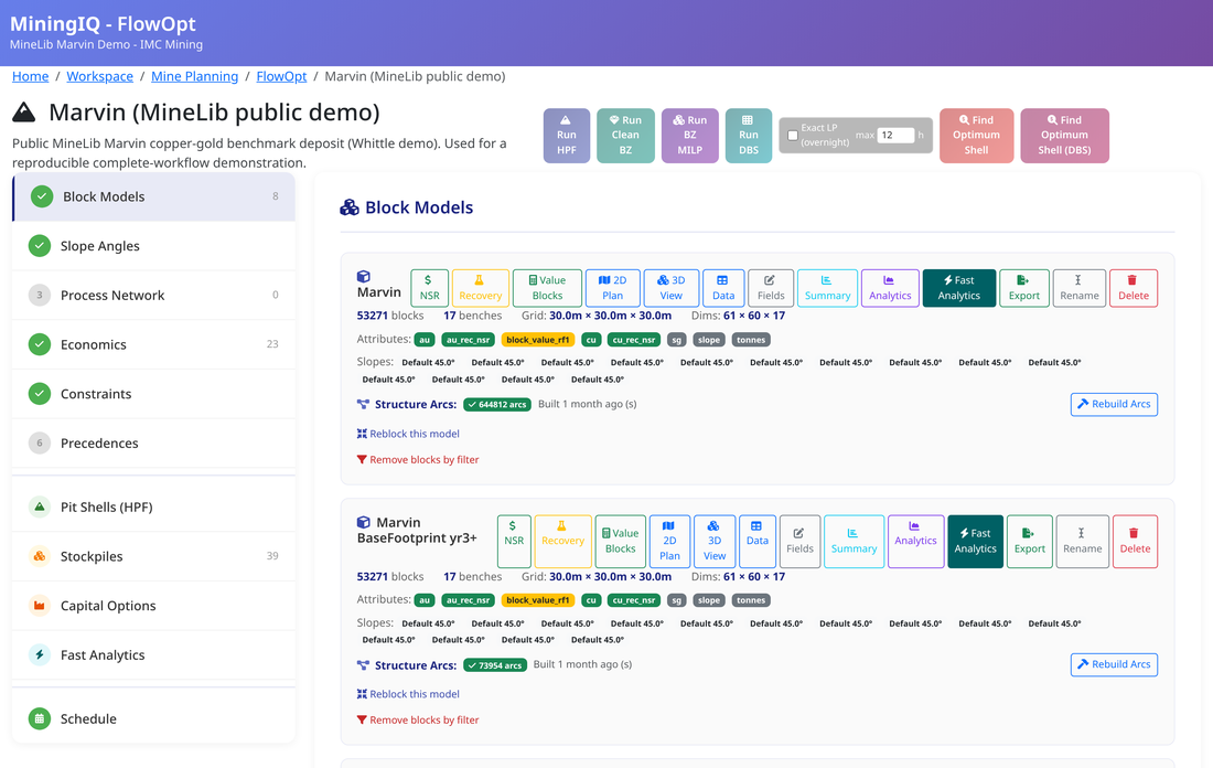
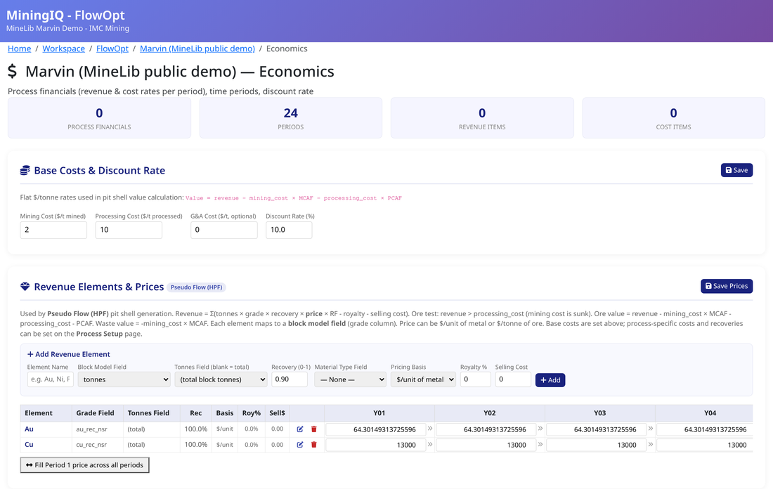
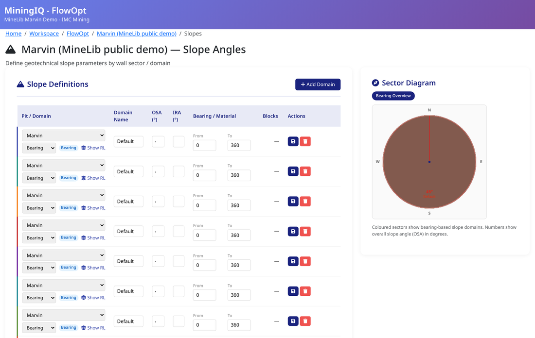
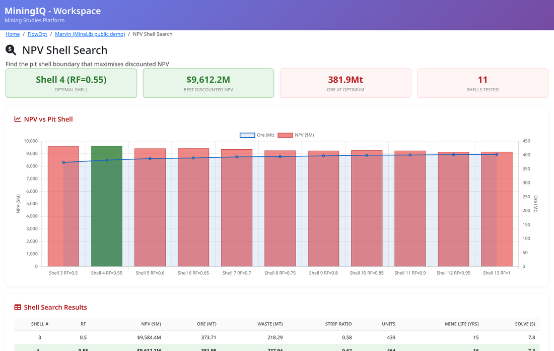
What it does
Provably optimal ultimate pit
Solves the maximum-closure problem exactly. The answer is the optimum for the economics and slopes you entered — there is no gap and nothing to tune.
Nested shells in one parametric pass
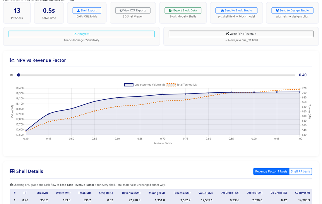
The full revenue-factor ladder is solved by reusing one flow network, so a 30-shell run costs a fraction of 30 separate solves — and the shells nest by construction.
Automated optimum-shell search
Sweeps revenue factors and reports the discounted best shell, so pit selection is a computed result rather than an eyeballed row in a table.
Reads your block model directly
Points straight at Datamine and Vulcan block models — no rebuilding the deposit in a separate optimiser format before you can run a case.
Geotechnically honest slopes
Azimuth–slope pairs interpolated around the pit, per-domain overrides, and correct cone geometry on non-cubic and sub-blocked models.
Full Whittle-grade economics
Metallurgical and mining recovery, dilution, separate ore and waste cost adjustment, ore-mining premium, royalties, TC/RC and per-block or per-column cut-off.
Straight into scheduling
The same precedence graph feeds the BZ scheduler and Direct Block Scheduling — the pit and the schedule are one continuous model, not two disconnected exercises.
Your team runs it, not us
Every client user has real-time access to the full interface and can set up and run their own cases, as many as they like, with no per-seat licence to pass around.
Implementation notesTechnical detail
The solver is a compiled C++17 pseudoflow engine (the MIT-licensed MineFlow library) bound to Python through pybind11, operating directly on NumPy arrays. Node and arc objects are pooled to keep allocation off the hot path, block values are scaled to 64-bit integers with overflow clamping, and precedence arc files are memory-mapped so graphs larger than RAM stream from disk.
Inputs are block values (or base revenue plus costs), grid dimensions, slope specification and block sizes, from CSV, .npy, or directly from Datamine and Vulcan block models. Output is an in-pit mask per revenue factor, plus the shell statistics and the NPV shell search.
- In
- block values (or base-revenue + costs), grid dims, slope, block sizes, revenue-factor list or explicit arcs; CSV or .npy.
- Out
- one in-pit boolean mask per revenue factor.
flowopt/services/mineflow_cpp/ · hpf_solver.py · slope_template.py · dbs_precedence.py
How our pseudoflow actually works
The problem
What the optimiser is actually solving
Pit optimisation looks like a geometry problem but is really a graph problem. Every block carries an economic value — what it is worth if you process it, minus what it costs to dig it. Some are positive, most are negative. You cannot take a positive block without first taking everything above it inside the slope cone.
That constraint makes the set of minable blocks a closure: if a block is in the pit, all of its predecessors must be too. The optimal pit is therefore the maximum-weight closure — the closed set whose block values sum to the largest possible total. That problem has an exact solution, and it is equivalent to finding a minimum cut on a flow network. No heuristics, no local optima, no operator judgement in the loop.
Build the graph
Add precedence as infinite-capacity arcs
Solve the min-cut with pseudoflow
Read the pit off the cut
Sweep the revenue factors — without rebuilding
Slope control
Precedence patterns — getting the cones right
The quality of a pit optimisation is decided by the precedence structure long before the solver runs. Approximating a slope cone with too coarse a pattern quietly costs you metres of wall angle across the whole pit.
The engine builds precedence from Caccetta–Giannini minimum-search patterns — the provably memory-minimal set of offsets that reproduces a given slope angle over a given number of benches. You get the geometric accuracy of a large search cone without carrying the arc count that would normally come with it.
Slopes that vary the way real pits do
Slopes are specified as azimuth–slope pairs and interpolated around the pit (linear, cubic or cosine), so a wall that steepens through a competent domain and lays back over a fault is represented as such — not averaged into a single overall angle. Block sizes are carried through the cone construction, so non-cubic blocks produce correct geometry rather than a distorted cone.
Irregular and sub-blocked models
Where a model is reblocked, sub-blocked or otherwise irregular, precedence can be supplied as an explicit arc list instead of a generated pattern. Those arc files are memory-mapped from disk, so a precedence graph far larger than RAM streams rather than loads — and the same arcs are what Direct Block Scheduling later schedules against.
Block valuation
The economics inside each block value
Before any graph is built, every block is valued through a full economic model — the same parameter set a Whittle practitioner would expect, because that is exactly the comparison our clients make:
- Metallurgical recovery per element, including recovery curves by material type
- Mining recovery and dilution applied to tonnes and grade
- Cost adjustment factors — separate ore and waste tables, varying by depth or domain
- Ore-mining premium for the additional cost of selective ore mining
- Royalties and TC/RC plus selling and transport costs
- Cut-off grade applied per block or per column, with ore-class masks for material routing
Values are converted to scaled 64-bit integers inside the solver, with overflow clamping, so the minimum cut is computed in exact integer arithmetic. Floating-point drift cannot quietly corrupt the optimum on a large deposit — a failure mode that is easy to miss precisely because the answer still looks plausible.
Optimum revenue factor
Finding the optimum shell, not just drawing shells
Producing 30 nested shells is the easy part. The question that actually matters is which one is the pit — and the largest shell is almost never the right answer, because the undiscounted ultimate pit ignores the fact that the last increment of stripping is paid for years before its ore is milled.
The system runs a revenue-factor search across the ladder, evaluates each candidate shell on a discounted basis rather than an undiscounted one, and reports the shell that maximises value along with the trade-off curve behind it. Pit selection becomes a computed, reproducible result you can defend in a review — not a judgement call about which row of a table looked best on the day.
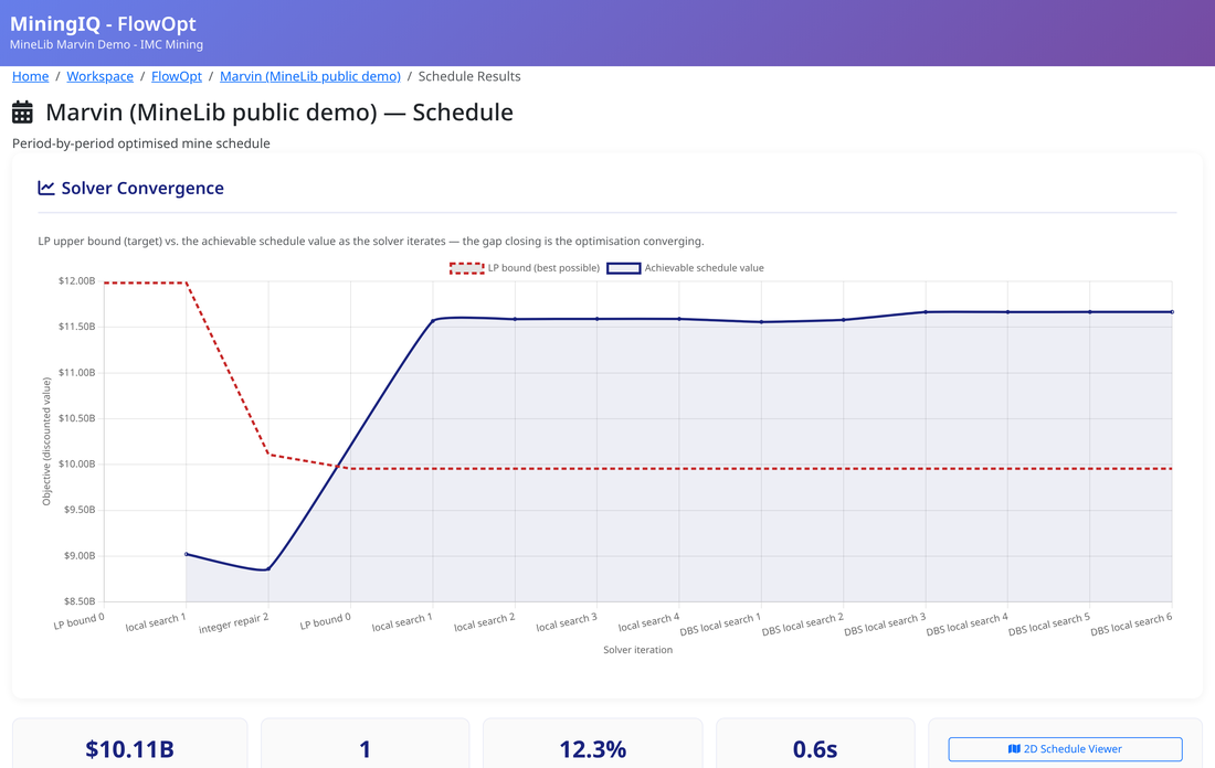
Direct Block Scheduling takes this further again: rather than accepting any shell as given, it runs the discounted schedule across the candidate shells and keeps the NPV-best precedence-closed pit. The pit is chosen by the schedule that will actually be mined.
Where we match, and where we go further
The conventional column describes the standard desktop pit-optimisation workflow most teams will recognise. Green rows are where we deliberately match it. The rest is what a connected, browser-based platform makes possible.
| Capability | Conventional workflow | MiningIQ |
|---|---|---|
| Ultimate pit algorithm | Lerchs–Grossmann, with pseudoflow in later versions — exact maximum closure. | Hochbaum pseudoflow in compiled C++ — the same exact optimum, validated shell by shell against Whittle. |
| Economic model | Recoveries, dilution, cost adjustment factors, royalties, TC/RC, cut-off. | The same parameter set, deliberately mirrored so results reconcile line for line. |
| Nested revenue-factor shells | Shell ladder generated per revenue factor. | One parametric pass reusing the flow network — the ladder costs a fraction of N separate solves. |
| Slope control | Slope sets by zone or azimuth. | Azimuth–slope pairs with interpolation, per-domain overrides, correct cones on non-cubic and sub-blocked models. |
| Block model input | Deposit is exported from the geology package and rebuilt in the optimiser's own model format. | Points directly at the Datamine or Vulcan block model — no intermediate model build, so no re-import every time geology updates. |
| Choosing the pit | Practitioner inspects the shell table and picks a pushback set by judgement. | Automated revenue-factor search reports the discounted-best shell, with the trade-off curve behind it. |
| Block-level scheduling | Shells become pushbacks, which are then scheduled by period. | Direct Block Scheduling schedules every block against the same geotechnical precedence — no pushback abstraction in between. |
| Development shells | Not part of the workflow. | The dig sequence is banded by cumulative mined ore into nested masks — a time-and-tonnage analogue of pit shells. |
| Cost basis | Costs arrive as assumptions from an external spreadsheet. | Zero-based MineCost engine builds capex and opex bottom-up and feeds the optimiser directly. |
| Value and risk | NPV computed downstream in a separate financial model. | Full three-statement DCF, valuation and P10/P50/P90 risk on the same platform, off the same schedule. |
| 3D and CAD outputs | Shell results returned to the mining package. | Interactive 3D viewer plus DXF export that lands directly in Leapfrog, Deswik and Vulcan. |
| Who can run it | Per-seat desktop licences, so runs queue behind whoever holds one. | Browser-based with real-time access for every client user — your team sets up and runs its own cases, unlimited. |
Downstream
What happens to the answer next
A pit shell that stops at a picture is only half a deliverable. Because the optimiser sits inside the platform rather than beside it, the result keeps moving:
- Into the scheduler — the same precedence graph drives the BZ scheduler and Direct Block Scheduling, so the pit and the mining sequence are one model.
- Into 3D — shells, benches and solids render interactively in the browser for review.
- Into your CAD packages — DXF export drops straight into Leapfrog, Deswik and Vulcan, alongside Datamine and Vulcan block-model writes.
- Into the money — tonnes and grades flow to the MineCost zero-based cost model and on into the financial model and risk analysis without a re-key.
And because it is a web platform, your own people do this — set up cases, run them, compare them, export them — in real time, without waiting on a consultant's licence seat or a returned deliverable.